# Packages
library(tidyverse)

# Today we will also be using
# This is helpful to check the assumptions of linear models
library(performance)3 Session 3: Linear regression
3.1 Preliminaries
- You should have created an
Rstudioproject in Week 1. If you have not do so yet, I encourage you to return to a previous chapter for detailed instructions on data availability and structure. - Get familiar with the dataset. If you haven’t do so, take a few minutes to look at the introduction to it is available at: https://www.psrc.org/media/3248, and the data dictionary, which is avaiable on Moodle, too.
For today’s session we will need the following packages. Install them using the install.packages() function if you don’t have them available.
Now, we will read the data in to the R session. We will use three tables from the travel survey dataset.
# Read data
trips <- read_csv('data/Trips.csv')
persons <- read_csv('data/Persons.csv')
households <- read_csv('data/Households.csv')
3.2 Estimating the average miles driven per household a day
In this first example, we are interested to know about driving behaviour. So, we will use the ‘trips’ table to summarise information, and supplement it with information from the ‘households’ table by joining these together.
First, we will subset the trips which primary trip mode is ‘Drive’ only, for the year 2023.
trips_drive <- trips %>%
  filter(grepl('Drive', mode_class) & survey_year == '2023')
What is function grepl() doing in the previous chunk? How many observations were kept in for trips driving compared to all of the trips?
The we will create key variables relating to driving behaviour at the household level. We are crucially interested in the average miles driven a day per household. To do so, we summarise the information at the household level. Effectively, we sum the trip distance, and divide it by the number of days with trips recorded in the survey to obtain the average miles driven.
miles_driven_hh <- trips_drive %>%
  group_by(household_id) %>%
  summarise(
    total_miles_hh = sum(distance_miles, na.rm = TRUE),
    num_days_trips = n_distinct(daynum),
    avg_miles_driven = total_miles_hh / num_days_trips
  )
As we now have a summary per household, we can join more information about the household using the ‘household_id’ unique identifier in the left_join() function.
# Join household data
miles_driven_hh <- miles_driven_hh %>%
  left_join(households, by = 'household_id')
3.3 Exploratory analysis
In this analysis, we will focus on respondents having more than 0 miles driven. In other words, only households who have reported to have droven in the survey.
# Subset
miles_driven_hh <- miles_driven_hh %>%
  filter(avg_miles_driven > 0)
Lte’s visualize distribution of miles driven.
miles_driven_hh %>%
  ggplot(aes(avg_miles_driven)) +
  geom_density() +
  labs(x = 'Avg. miles driven per household', y = 'Density') +
  theme_minimal()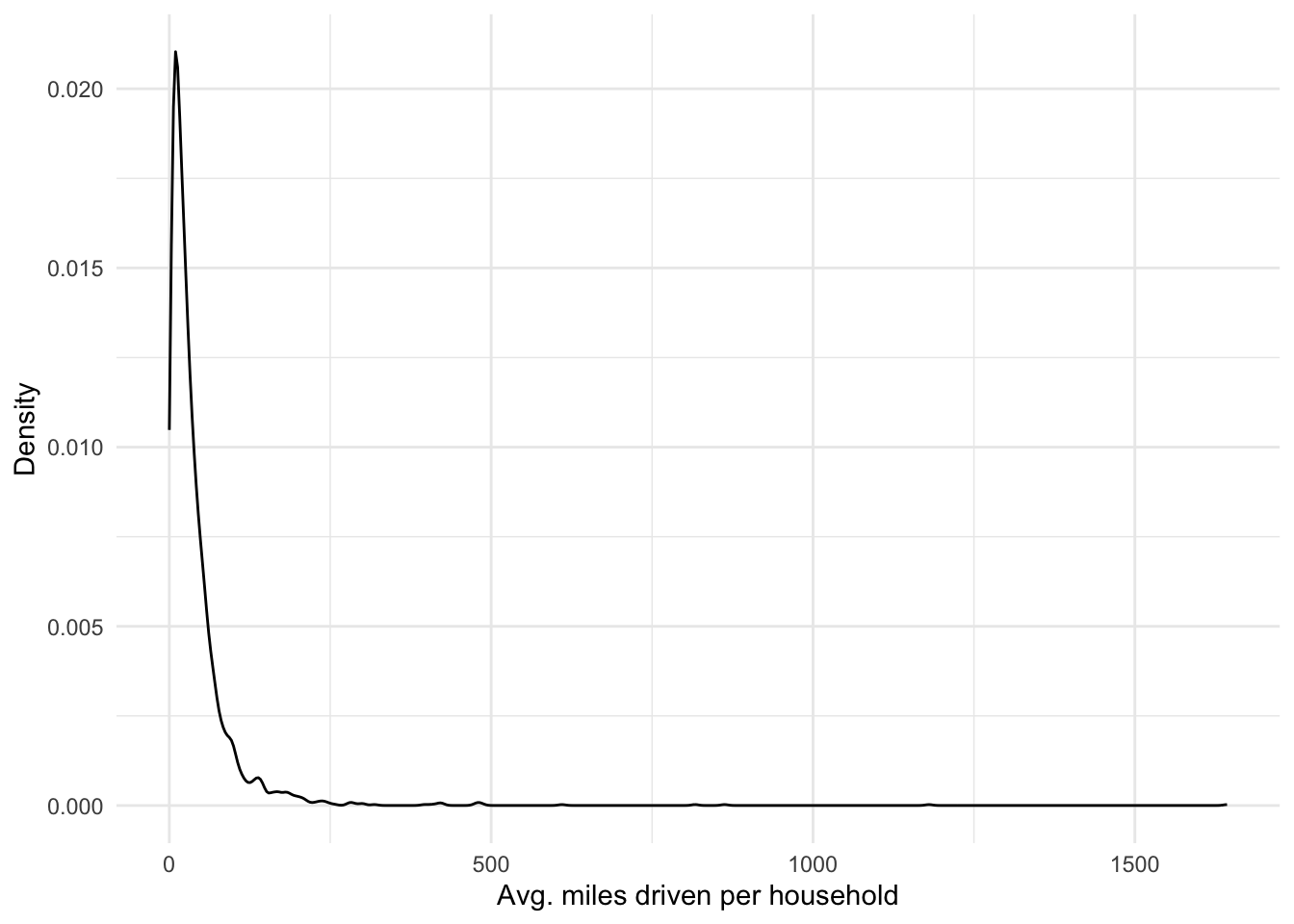
Something strange?…
Let’s limit the maximum average of vehicle miles driven. The threshold chosen should be justified, e.g. preliminary information in the context, literature, or external empirical references.
miles_driven_hh <- miles_driven_hh %>%
  filter(avg_miles_driven <= 500)
3.3.1 Bivariate analysis
We will transform the numchildren variables to factor, treating it as a categorical. Why? Are there options?
miles_driven_hh <- miles_driven_hh %>%
  mutate(numchildren = factor(numchildren))
Plot the distribution of the average vehicle miles driven by groups.
# Plot distribution by groups
miles_driven_hh %>%
  ggplot(aes(numchildren, avg_miles_driven)) +
  geom_boxplot() +
  labs(x = 'Number of children', y = 'Avg. miles driven per household') +
  theme_minimal()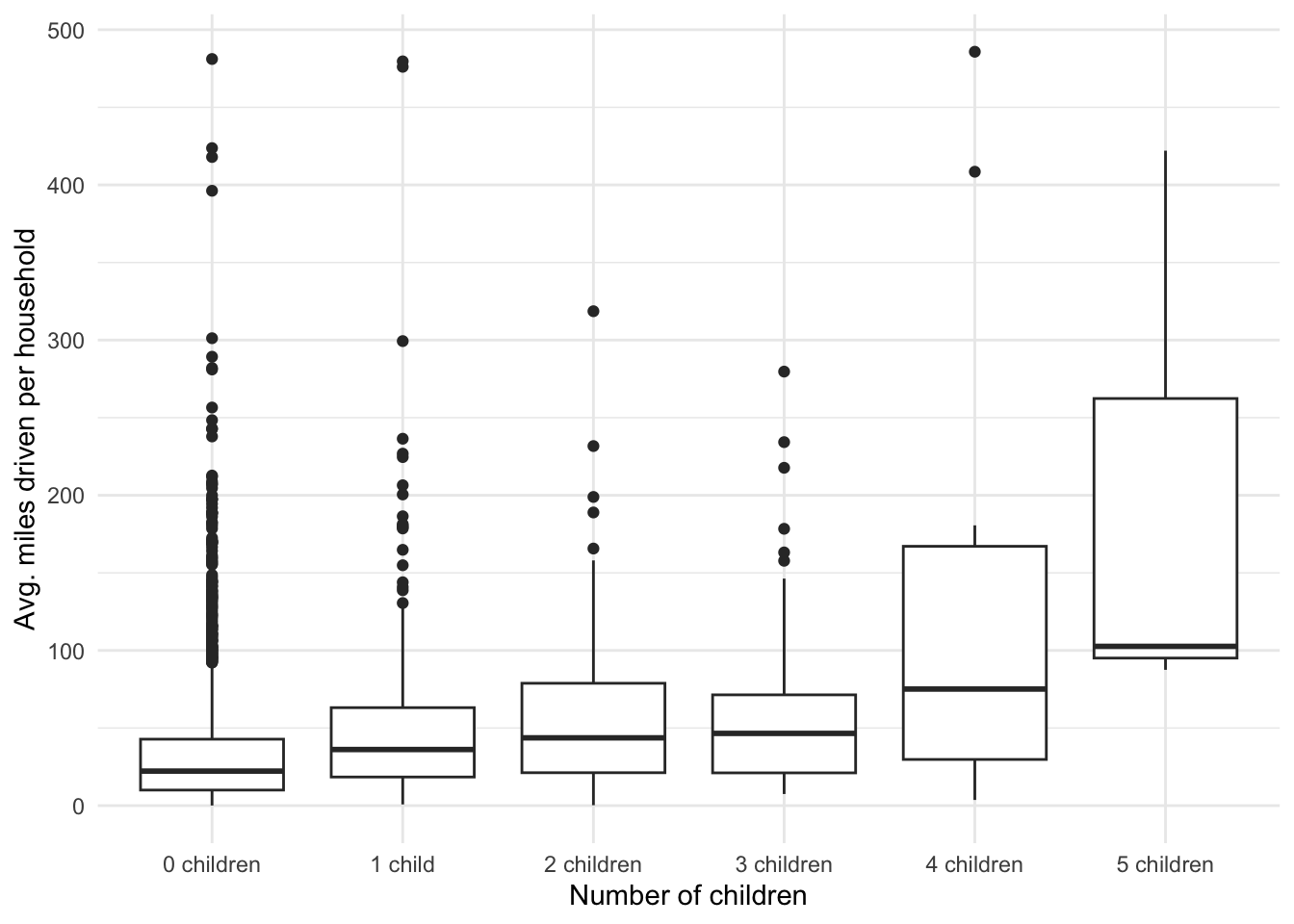
3.3.2 How does working from home relates to vehicle miles driven?
In this session, the aim is to explain wow working from home relates to vehicle miles driven. For this, we will need to get the information about individuals in the household. We can do this using the ‘persons’ table.
First, look at the categories in the ‘workplace’ variable
count(persons, workplace)# A tibble: 7 × 2
workplace n
<chr> <int>
1 At home (telecommute or self-employed with home office) 2118
2 Drives for a living (e.g., bus driver, salesperson) 257
3 Missing: Skip Logic 7652
4 Telework some days and travel to a work location some days 1554
5 Usually the same location (outside home) 8184
6 Workplace regularly varies (different offices or jobsites) 1519
7 <NA> 2366Then, we create a new binary variable which identifies people working from home.
# Create a binary variable indicating if anyone in works from home or teleworks
persons <- persons %>%
  mutate(
    work_from_home =
      ifelse(
        # If the variable workplace contains 'At home' or 'Telework'
        grepl('At home|Telework', workplace),
        # return 'Yes'.
        'Yes',
        # Otherwise, we set it to 'No'
        'No'
))
To help you going about the previous code, you can read for more information about the conditional function typing ?ifelse in your R console.
Then, we summarise the information at the household level summing the number of individuals at the household which work from home (‘pers_work_home’). Also, we will create another variable which checks if at leas one person works from home, i.e. ‘work_from_home’.
work_from_home <- persons %>%
  group_by(household_id) %>%
  summarise(
    pers_work_home = sum(work_from_home == 'Yes', na.rm = TRUE),
    any_work_home = ifelse(pers_work_home > 0, 'Yes', 'No')
  )
Now, we can join this new information to the data at the household level.
# Join to subset
miles_driven_hh <- miles_driven_hh %>%
  left_join(work_from_home, by = 'household_id')
Is there any visual difference at the household level?
# Visualise
miles_driven_hh %>%
  ggplot(aes(any_work_home, avg_miles_driven)) +
  geom_boxplot() +
  labs(
    x = 'Any working from home',
    y = 'Avg. miles driven per household'
  ) +
  theme_minimal()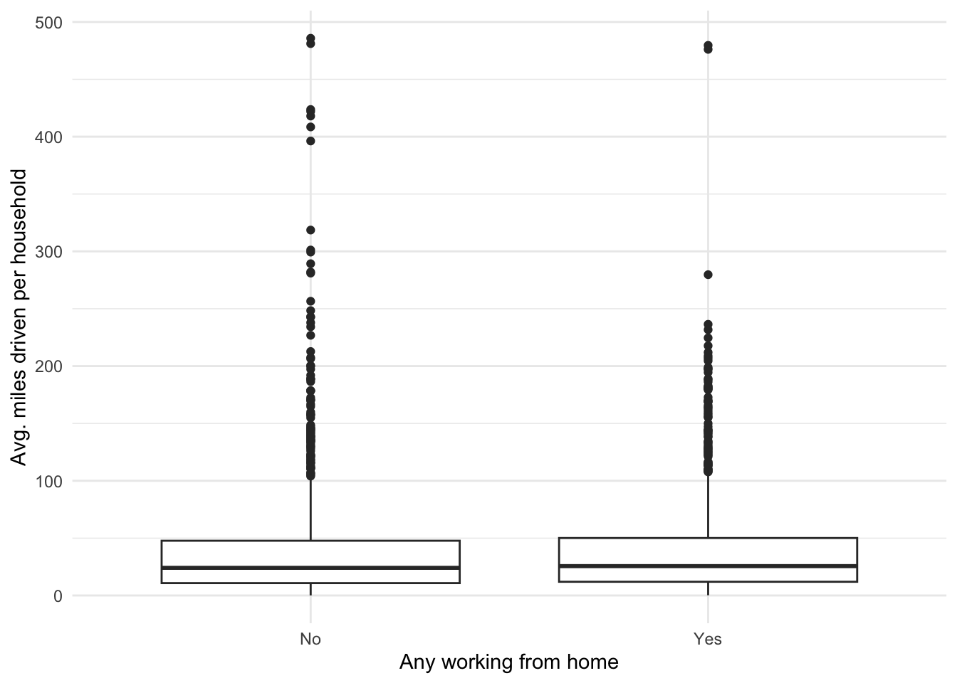
What about the descriptive statistics?
miles_driven_hh %>%
  group_by(any_work_home) %>%
  summarise(
    miles_driven_mean = mean(avg_miles_driven),
    miles_driven_sd = sd(avg_miles_driven)
  )
# A tibble: 2 × 3
any_work_home miles_driven_mean miles_driven_sd
<chr> <dbl> <dbl>
1 No 38.4 48.5
2 Yes 38.7 42.73.4 Evaluate the difference in a linear regression analysis
Let’ see what a simple linear model suggest.
miles_driven_hh %>%
  lm(avg_miles_driven ~ any_work_home, .) %>%
  summary()
Call:
lm(formula = avg_miles_driven ~ any_work_home, data = .)

Residuals:
   Min     1Q Median     3Q    Max
-38.53 -27.34 -13.47   9.98 447.39

Coefficients:
                 Estimate Std. Error t value Pr(>|t|)
(Intercept)       38.4147     1.1645  32.989   <2e-16 ***
any_work_homeYes   0.3259     1.7349   0.188    0.851
---
Signif. codes:  0 '***' 0.001 '**' 0.01 '*' 0.05 '.' 0.1 ' ' 1

Residual standard error: 45.99 on 2837 degrees of freedom
Multiple R-squared:  1.244e-05, Adjusted R-squared:  -0.00034
F-statistic: 0.03528 on 1 and 2837 DF,  p-value: 0.851
Are there potential problems with this model or results?
We will add socio-demographic variables as controls, e.g. size of the household matters!
First, we format the order of household income labels and convert size of household from character to numeric. This will ease interpretations.
# Income labels
income_labs <- c(
  "Under $25,000",
  "$25,000-$49,999",
  "$50,000-$74,999",
  "$75,000-$99,999",
  "$100,000-$199,999",
  "$200,000 or more"
)
miles_driven_hh <- miles_driven_hh %>%
  mutate(
    # Income labels
    hhincome_broad = factor(hhincome_broad, income_labs),
    # Household size as integer
    hhsize_int = readr::parse_number(hhsize, "\\d+"),
    # Children at household as binary
    children_binary = ifelse(numchildren == '0 children', 'No', 'Yes')
)
We run the multiple regression and print results.
m1 <- miles_driven_hh %>%
  lm(
    avg_miles_driven ~
      any_work_home + hhsize_int + hhincome_broad + children_binary, .
  )
summary(m1)
Call:
lm(formula = avg_miles_driven ~ any_work_home + hhsize_int +
    hhincome_broad + children_binary, data = .)

Residuals:
   Min     1Q Median     3Q    Max
-85.49 -23.42 -10.93   9.53 433.53

Coefficients:
                                Estimate Std. Error t value Pr(>|t|)
(Intercept)                        7.253      3.661   1.981 0.047702 *
any_work_homeYes                  -7.782      1.961  -3.969 7.43e-05 ***
hhsize_int                        10.390      1.099   9.451  < 2e-16 ***
hhincome_broad$25,000-$49,999      6.121      4.128   1.483 0.138285
hhincome_broad$50,000-$74,999     13.564      4.031   3.365 0.000778 ***
hhincome_broad$75,000-$99,999     10.066      4.163   2.418 0.015682 *
hhincome_broad$100,000-$199,999   18.768      3.770   4.978 6.84e-07 ***
hhincome_broad$200,000 or more    13.923      4.112   3.386 0.000721 ***
children_binaryYes                 1.522      3.137   0.485 0.627681
---
Signif. codes:  0 '***' 0.001 '**' 0.01 '*' 0.05 '.' 0.1 ' ' 1

Residual standard error: 45.08 on 2562 degrees of freedom
  (268 observations deleted due to missingness)
Multiple R-squared:  0.09071,   Adjusted R-squared:  0.08787
F-statistic: 31.95 on 8 and 2562 DF,  p-value: < 2.2e-16
Discuss the model results with your tutor.
3.5 Does it meet the model assumptions? … Lets check the model
Check model 1 assumptions. Type ‘y’ when you are asked about updating extensions.
check_model(m1)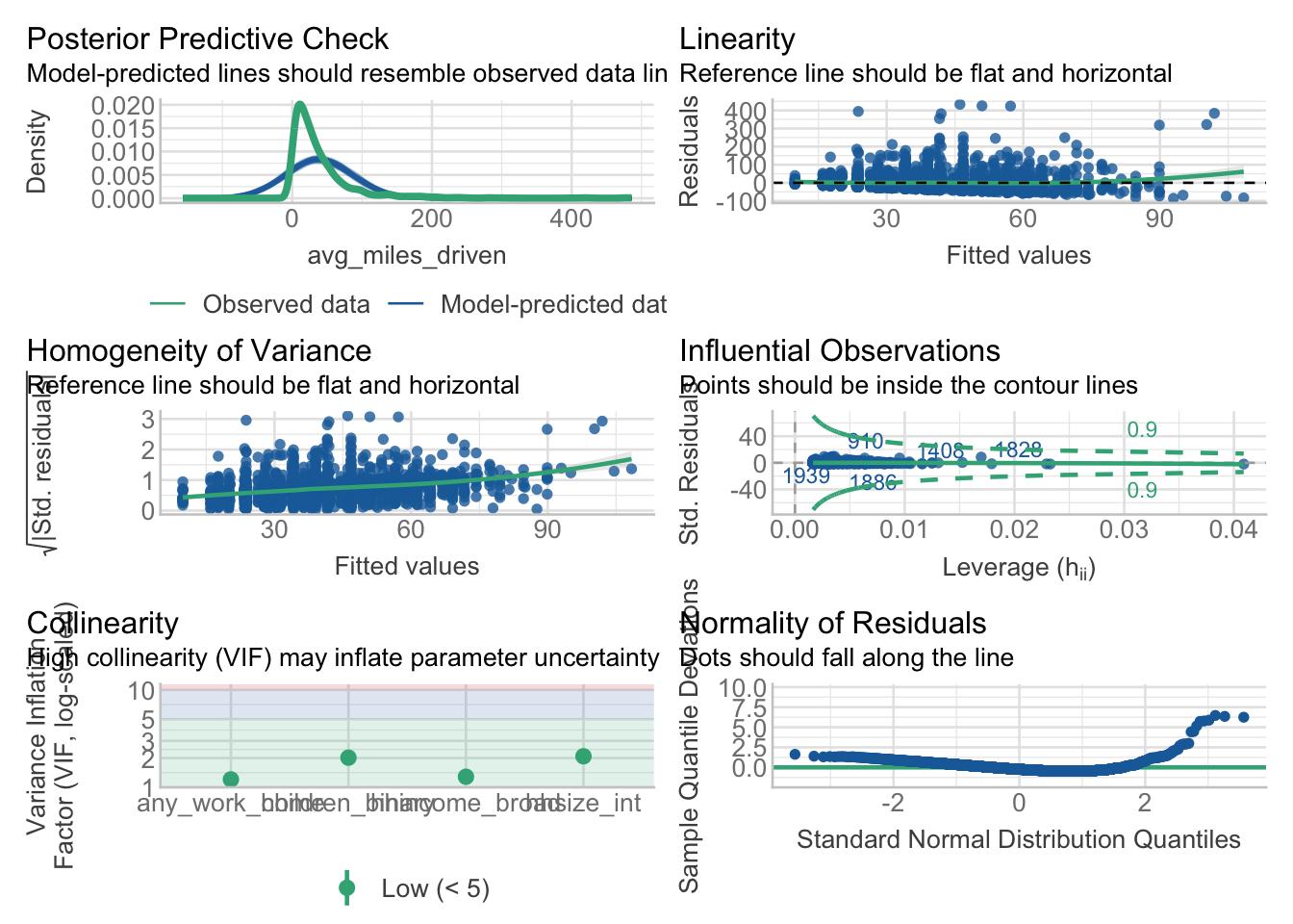
3.6 A log-linear model
Lets try to fit the model in the log-linear form.
m2 <- miles_driven_hh %>%
  mutate(log_miles_driven = log(avg_miles_driven)) %>%
  lm(
    log_miles_driven ~
      any_work_home + hhsize_int + hhincome_broad + children_binary, .
)
And check the model again
check_model(m2)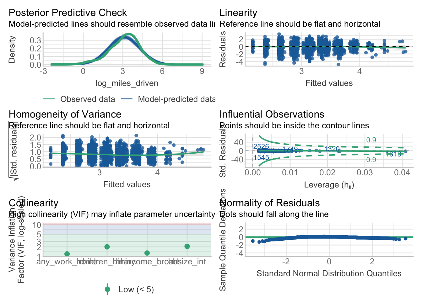
What are the interpretations of the log-linear model? Think of coefficients and overall performance.
summary(m2)
Call:
lm(formula = log_miles_driven ~ any_work_home + hhsize_int +
    hhincome_broad + children_binary, data = .)

Residuals:
    Min      1Q  Median      3Q     Max
-4.8991 -0.6340  0.1017  0.7374  3.4246

Coefficients:
                                Estimate Std. Error t value Pr(>|t|)
(Intercept)                      2.10369    0.08813  23.872  < 2e-16 ***
any_work_homeYes                -0.21061    0.04720  -4.462 8.46e-06 ***
hhsize_int                       0.26492    0.02646  10.012  < 2e-16 ***
hhincome_broad$25,000-$49,999    0.24219    0.09936   2.437   0.0149 *
hhincome_broad$50,000-$74,999    0.50126    0.09704   5.166 2.58e-07 ***
hhincome_broad$75,000-$99,999    0.49212    0.10021   4.911 9.63e-07 ***
hhincome_broad$100,000-$199,999  0.71162    0.09074   7.843 6.42e-15 ***
hhincome_broad$200,000 or more   0.65926    0.09899   6.660 3.33e-11 ***
children_binaryYes               0.01942    0.07551   0.257   0.7971
---
Signif. codes:  0 '***' 0.001 '**' 0.01 '*' 0.05 '.' 0.1 ' ' 1

Residual standard error: 1.085 on 2562 degrees of freedom
  (268 observations deleted due to missingness)
Multiple R-squared:   0.12, Adjusted R-squared:  0.1173
F-statistic: 43.68 on 8 and 2562 DF,  p-value: < 2.2e-16
Which model would you choose? Are the any other potentially omitted variables?
4 Individual activities
- Estimate average miles at the household level for a different mode, e.g. transit, bike, walk, etc.
- How does having children relates to the observed behaviour after controlling for important socio-demographic variables? Include descriptive statistics, plots, and multiple linear regression analysis.
- Try different functional forms.
- To what extent are the assumptions of the linear model met?