library(tidyverse) # for data manipulation and visualization2 Session 2 Data structures and descriptive statistics
2.1 Preliminaries
First, load the packages required for the analysis (install if needed).
We will pick it up where we left it last time, and read the household data in the RDS file you prepared. If you haven’t completed Session 1, go to it and complete it before continuing here.
household_subset <- read_rds('data/household_subset.RDS')You will also need the ‘Trips’ table for this session. As we will combine the information from households and trips reported by each household.
trips <- read_csv("data/Trips.csv")2.2 Format Trips table
Subset trips for the year 2023 and keep only variables of interest.
trips_subset <- trips %>%
  filter(survey_year == 2023) %>%
  select(
    household_id, person_id, trip_id,
    mode_class, depart_date, depart_time_hour,
    arrival_time_hour, origin_county, dest_county,
    origin_purpose_cat, dest_purpose_cat, distance_meters,
    duration_minutes
)
ALWAYS CHECK THE SUBSET!!! What would you check?
nrow(trips_subset)[1] 56704ncol(trips_subset)[1] 13colnames(trips_subset) [1] "household_id" "person_id" "trip_id"
[4] "mode_class" "depart_date" "depart_time_hour"
[7] "arrival_time_hour" "origin_county" "dest_county"
[10] "origin_purpose_cat" "dest_purpose_cat" "distance_meters"
[13] "duration_minutes" head(trips_subset)# A tibble: 6 × 13
household_id person_id trip_id mode_class depart_date depart_time_hour
<dbl> <dbl> <dbl> <chr> <date> <dbl>
1 23000858 2300085801 2300085801002 Walk 2023-04-27 16
2 23000466 2300046601 2300046601004 Walk 2023-04-20 14
3 23001235 2300123501 2300123501011 Drive HOV3+ 2023-04-27 19
4 23000466 2300046601 2300046601005 Walk 2023-04-20 14
5 23000858 2300085801 2300085801003 Drive HOV2 2023-04-27 19
6 23001235 2300123501 2300123501012 Drive HOV3+ 2023-04-27 19
# ℹ 7 more variables: arrival_time_hour <dbl>, origin_county <chr>,
# dest_county <chr>, origin_purpose_cat <chr>, dest_purpose_cat <chr>,
# distance_meters <dbl>, duration_minutes <dbl>Transform the categorical variables as factor.
trips_subset <- trips_subset %>%
  mutate(
    across(
      c(mode_class, origin_county, dest_county, origin_purpose_cat, dest_purpose_cat),
      as.factor)
  )
2.3 Trip descriptive statistics
Calculate a summary at the person-level. Include the number of trips, total travel distance and travel time for each person, within household.
person_summary <- trips_subset %>%
  group_by(person_id, household_id) %>%
  summarise(
    number_of_trips = n(),
    # Distance in kilometres
    total_travel_distance = sum(distance_meters / 1000),
    total_travel_time = sum(duration_minutes)
  ) %>%
  ungroup()
Now, you need to normalise the total distance and travel time based on the number of trips by calculating the average values.
person_summary <- person_summary %>%
  mutate(
    avg_trip_distance = total_travel_distance / number_of_trips,
    avg_trip_duration = total_travel_time / number_of_trips
  )
Create a quick summary
summary(person_summary) person_id household_id number_of_trips total_travel_distance
Min. :2.300e+09 Min. :23000173 Min. : 2.000 Min. : 0.066
1st Qu.:2.307e+09 1st Qu.:23070124 1st Qu.: 2.000 1st Qu.: 11.425
Median :2.315e+09 Median :23153760 Median : 4.000 Median : 29.122
Mean :2.317e+09 Mean :23170889 Mean : 9.509 Mean : 124.803
3rd Qu.:2.326e+09 3rd Qu.:23264171 3rd Qu.: 8.000 3rd Qu.: 79.841
Max. :2.342e+09 Max. :23423045 Max. :307.000 Max. :18795.769
NA's :1
total_travel_time avg_trip_distance avg_trip_duration
Min. : 2.0 Min. : 0.033 Min. : 1.00
1st Qu.: 48.0 1st Qu.: 2.925 1st Qu.: 12.97
Median : 88.0 Median : 5.951 Median : 19.00
Mean : 196.7 Mean : 14.324 Mean : 24.67
3rd Qu.: 205.0 3rd Qu.: 12.080 3rd Qu.: 30.00
Max. :2573.0 Max. :2697.030 Max. :270.50
NA's :1 NA's :1 NA's :1 Do the values make sense?
There are some extreme values in the number of trips (more than 300?!) and average trip distance (more thank 2,000 KM?). We will remove them for this analysis. In practice, we should carefully make choices and justify them.
person_summary <- person_summary %>%
  filter(number_of_trips < 50 & avg_trip_distance < 100)
3 Joining tables
Join the household information to person summary.
person_summary <- left_join(person_summary, household_subset, by = "household_id")- Why do we join by ‘household_id’?
- Have a look to the result. What do you observe? What is the observation unit? Does it make sense?
glimpse(person_summary)Rows: 5,775
Columns: 15
$ person_id <dbl> 2300017301, 2300017302, 2300017303, 2300017304, …
$ household_id <dbl> 23000173, 23000173, 23000173, 23000173, 23000213…
$ number_of_trips <int> 21, 5, 2, 37, 5, 3, 37, 24, 2, 16, 19, 2, 2, 4, …
$ total_travel_distance <dbl> 160.115165, 30.995001, 6.699998, 185.559998, 9.3…
$ total_travel_time <dbl> 605, 96, 25, 551, 110, 39, 631, 514, 35, 621, 55…
$ avg_trip_distance <dbl> 7.624532, 6.199000, 3.349999, 5.015135, 1.866000…
$ avg_trip_duration <dbl> 28.80952, 19.20000, 12.50000, 14.89189, 22.00000…
$ hhincome_broad <fct> "$100,000-$199,999", "$100,000-$199,999", "$100,…
$ hhsize <dbl> 4, 4, 4, 4, 3, 2, 3, 3, 1, 1, 1, 2, 2, 2, 2, 1, …
$ home_county <fct> Kitsap County, Kitsap County, Kitsap County, Kit…
$ vehicle_count <dbl> 3, 3, 3, 3, 0, 2, 1, 1, 1, 1, 0, 1, 1, 2, 2, 2, …
$ hh_race_category <fct> White non-Hispanic, White non-Hispanic, White no…
$ numadults <dbl> 2, 2, 2, 2, 3, 2, 2, 2, 1, 1, 1, 2, 2, 2, 2, 1, …
$ numchildren <dbl> 2, 2, 2, 2, 0, 0, 1, 1, 0, 0, 0, 0, 0, 0, 0, 0, …
$ numworkers <dbl> 2, 2, 2, 2, 3, 0, 0, 0, 1, 1, 1, 2, 2, 2, 2, 1, …3.1 Visualising data
Univariate distribution: Check number of trips.
person_summary %>%
  ggplot(aes(number_of_trips)) +
  geom_histogram() +
  labs(
    x = "Total number of trips",
    y = "Count"
  )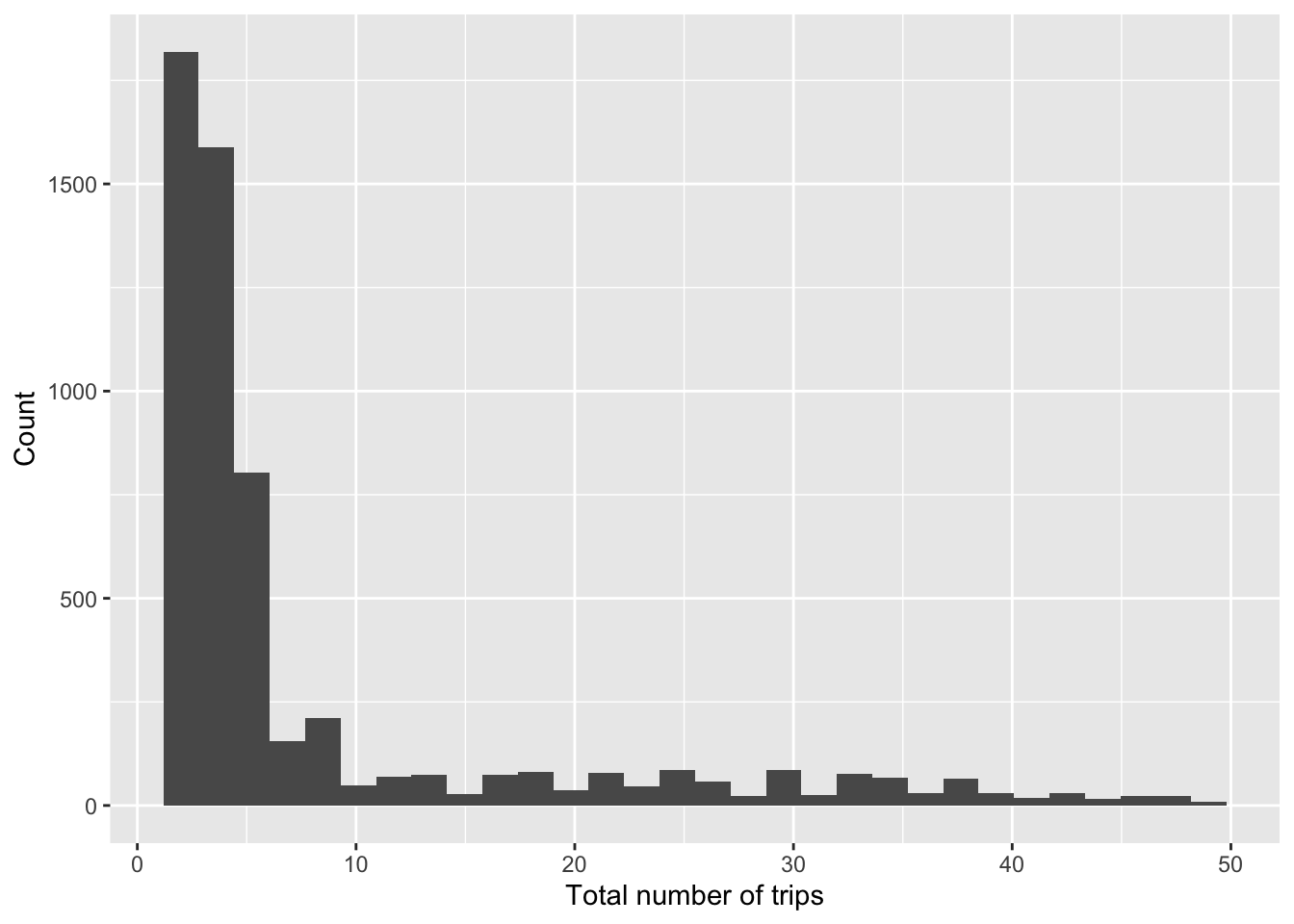
What is a suitable alternative to a histogram to visualise a variable distribution?
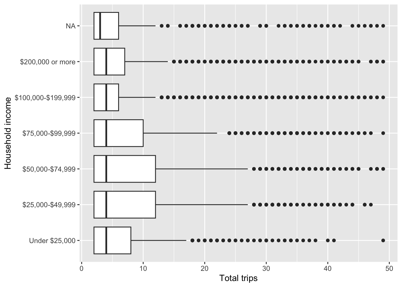
Bivariate plot: Visualise average number of trip and HH income.
person_summary %>%
  ggplot(aes(number_of_trips, hhincome_broad)) +
  geom_boxplot() +
  labs(
    x = "Total trips",
    y = "Household income"
  )
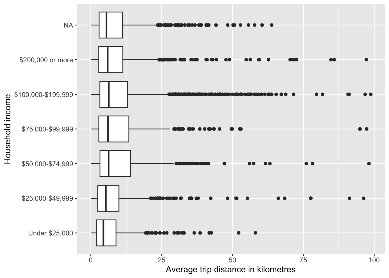
Visualise average trip distance and HH income.
person_summary %>%
  ggplot(aes(avg_trip_distance, hhincome_broad)) +
  geom_boxplot() +
  labs(
    x = "Average trip distance in kilometres",
    y = "Household income"
  )
4 Individual activities
- Read the Persons table.
- Filter out year
20212023 and select some variables of interest, e.g. household_id, person_id, employment, education, age, commute_freq, mode of transport for work. - Transform the selected columns to factors when appropriate.
- Join the household subset data.
- Summarise and visualise the key variables of your choice. (Note: focus on just a few selected key variables, yo do not need to visualise each of the selected ones).